Predicting Car Sales in Indonesia Using Long Short-Term Memory and Gated Recurrent Unit Algorithms
Abstract — Predicting car sales in Indonesia provides valuable insights into the country's automotive market and economic trends. This study evaluates and compares two deep learning models— Long Short-Term Memory (LSTM) and Gated Recurrent Unit (GRU)—to predict domestic car sales. Using historical sales data from GAIKINDO alongside macroeconomic indicators from BPS, Trading Economics, Kemendag, and Bank Indonesia, both models were tested across standard evaluation metrics (MAE, MSE, RMSE, and MAPE). The GRU model outperformed LSTM, achieving a lower average error rate of 12.49% compared to 12.56%. To make these insights accessible, the final predictive pipeline was deployed into an interactive web dashboard.
Keywords — Prediction; Sales; Cars; Long Short-Term Memory; Gated Recurrent Unit; Fine-Tuning; Evaluation Metrics
I. Introduction
II. Methodology
A. Data Acquisition & Preprocessing
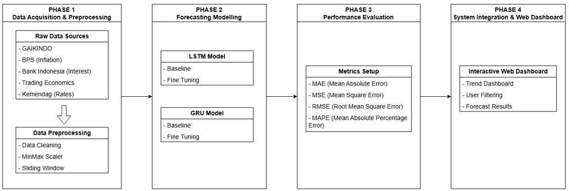
The study combines automotive sales records with macroeconomic statistics spanning 2015 to 2025. Monthly passenger car sales records were obtained from the Indonesian Automotive Industry Association (GAIKINDO) [3]. Macroeconomic variables—including inflation rates from the Central Statistics Agency (BPS), exchange rates from the Ministry of Trade (Kemendag), interest rates from Bank Indonesia, and fuel prices—were collected from Trading Economics. During preprocessing, data cleaning removed unused features and zero-sales records. The dataset was reshaped from a wide to a long format and integrated into a relational MySQL database. To prepare the data for recurrent neural networks, MinMax scaling normalized feature values, and a sliding window technique formatted the time-series data for supervised learning [4]. Before model training, exploratory data analysis via Pearson correlation assessed linear relationships between monthly car sales and macroeconomic indicators. The resulting heatmap matrix justified including these multivariate features in the prediction models [5]. Python served as the primary development platform, utilizing TensorFlow and Keras for model execution and Streamlit for web dashboard integration [6].
B. Proposed Prediction Models and Evaluation
The prediction phase evaluated two recurrent neural network architectures: Long Short-Term Memory (LSTM) and Gated Recurrent Unit (GRU). Model training followed a two-step approach: baseline testing to establish a benchmark, followed by hyperparameter fine-tuning (adjusting hidden units, batch size, learning rate, and network layer configurations) to maximize prediction accuracy. A critical parameter in time-series prediction is the lookback window, which defines the historical data span fed into the network. An appropriately tuned lookback window filters out historical noise and optimizes performance [7]. To evaluate different temporal dynamics, four lookback window scenarios were tested: 3 months (short-term), 6 months (medium-term), 12 months (annual seasonality), and 24 months (long-term). Model performance was evaluated across four standard metrics: MAE, MSE, RMSE, and MAPE [8].
C. System Integration and Web Dashboard
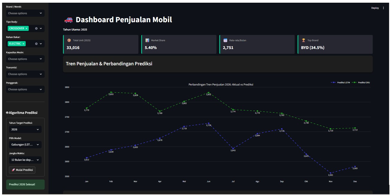
To provide interactive access to the prediction results, the top-performing model was deployed into a Streamlit-based web application. The dashboard automatically fetches trained models and dataset records from the MySQL database. Users can dynamically filter predictions by vehicle segment, brand, and fuel type to explore detailed automotive sales trends in Indonesia.
III. Results and Discussion
Feature Correlation Analysis
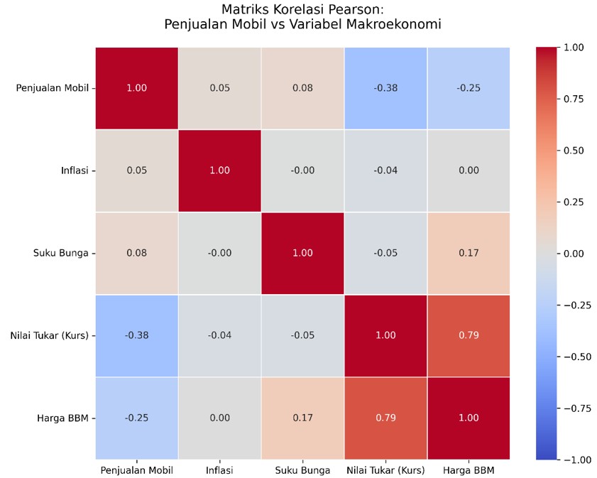
Exploratory data analysis using Pearson correlation assessed linear relationships between GAIKINDO vehicle sales data and key macroeconomic indicators, including fuel prices, general inflation, interest rates, and the Rupiah exchange rate. Pearson correlation coefficients range from -1 to 1, where values closer to -1 or 1 reflect strong linear relationships and values near 0 indicate weak ones. Figure 4 presents these bivariate relationships in a correlation matrix heatmap. As shown in Figure 4, car sales exhibit moderate negative correlations with the exchange rate (-0.38) and fuel prices (-0.25). These figures indicate an inverse relationship: Rupiah depreciation and rising fuel costs correlate with lower sales volumes. In contrast, car sales show negligible positive correlations with inflation (0.05) and interest rates (0.08), suggesting minimal direct linear impact on overall vehicle sales. Despite their weak linear relationship, inflation and interest rates were retained in the dataset. Advanced deep learning architectures, such as LSTM and GRU, excel at capturing complex non-linear patterns and temporal dependencies that standard Pearson correlation might miss. Consequently, all macroeconomic features were used for model training, with performance thoroughly evaluated in the following section.
Model Performance
To find the ideal historical data window for prediction, we evaluated lookback periods of 3, 6, 12, and 24 months. The 6-month window consistently produced the lowest error rates for both LSTM and GRU models, making it the baseline for further optimization. After baseline testing, we fine-tuned the model hyperparameters using a grid search. The optimal configuration for both architectures consisted of 256 hidden units, a batch size of 32, a standard network structure, and a learning rate of 0.0005. Table 2 summarizes the final performance metrics for the optimized models. As shown in Table 2, both models effectively captured automotive sales trends. However, the GRU architecture performed superiorly across all metrics, achieving the lowest MAE (5,800.46), RMSE (7,828.31), and a strong MAPE of 12.49%. This advantage stems from GRU’s streamlined gating mechanism, which efficiently captures non-linear patterns and temporal dependencies in multivariate sales data—resulting in an average monthly error margin of roughly 7,828 vehicle units.
| Model | MAE | MSE | RMSE | MAPE |
|---|---|---|---|---|
| LSTM | 5,994.03 | 69,248,438.64 | 8,321.56 | 12.56% |
| GRU | 5,800.46 | 61,282,488.23 | 7,828.31 | 12.49% |
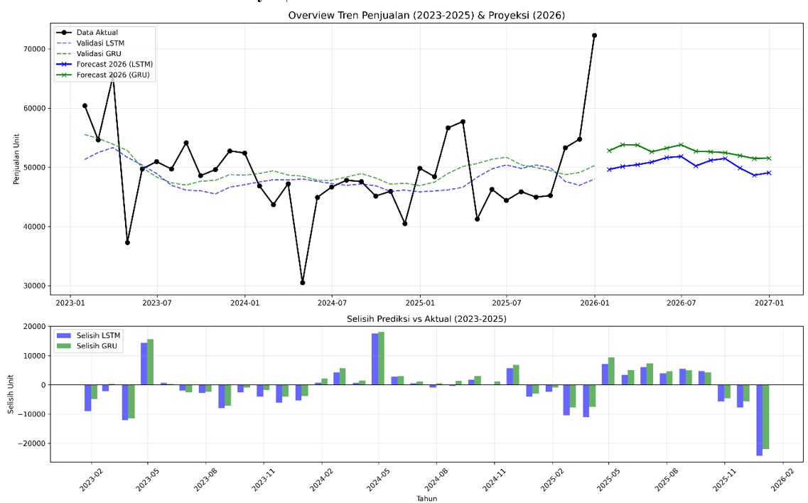
| Month (2026) | LSTM Prediction (Units) | GRU Prediction (Units) |
|---|---|---|
| January | 49,620 | 52,791 |
| February | 50,128 | 53,807 |
| March | 50,422 | 53,733 |
| April | 50,869 | 52,594 |
| May | 51,621 | 53,219 |
| June | 51,826 | 53,787 |
| July | 50,209 | 52,697 |
| August | 51,162 | 52,608 |
| September | 51,467 | 52,460 |
| October | 49,858 | 51,970 |
| November | 48,649 | 51,473 |
| December | 49,067 | 51,527 |