Layer Selection for Balanced Partial Federated Learning in Vehicular Networks
Chaehyeon Kim*, Computer Science and Engineering, Kyungpook National University
Daegu, Korea (south), hyeon917@knu.ac.kr
Youngjoon Yang*, Computer Science and Engineering, Kyungpook National University
Daegu, Korea (south), youngj719@knu.ac.kr
Seungwoo Lee*, Computer Science and Engineering, Kyungpook National University
Daegu, Korea (south), tmdrhdqn@knu.ac.kr
Dongkyun Kim*, Computer Science and Engineering, Kyungpook National University
Daegu, Korea (south), dongkyun@knu.ac.kr
* Corresponding author
Abstract — In federated learning (FL), the vehicles participating in training differ in their computational resources, so that the server must wait for the slowest vehicle to complete local training before aggregation. Consequently, the aggregation delay increases. Partial training, in which only a subset of the model layers is trained, reduces the aggregation delay. However, some layers are trained solely on the data of a few high-capability devices, which biases the model toward their data. In this paper, we propose a scheme in which each vehicle trains a contiguous layer interval that can be completed within a deadline and, in order to keep the per-layer training counts balanced, selects with a higher probability the intervals containing less frequently trained layers. Since interval selection and record management are performed by the vehicles, the server only performs aggregation. Simulation results on a real-world driving dataset show that the proposed scheme reduces the upload time per round compared with full-model training and achieves higher layer-wise training fairness than existing partial training schemes.
With the growing interest in autonomous driving, the ability of a vehicle to recognize surrounding objects has become increasingly important. An autonomous vehicle recognizes various objects, such as vehicles, pedestrians, and motorcycles, from the images captured by its cameras and determines its driving path and speed based on the recognition results. Since object recognition performance is directly related to safety, diverse objects must be recognized accurately. However, each vehicle typically drives in particular regions and time periods, and thus the data collected by each vehicle covers only a limited range of traffic environments. Therefore, the data collected by other vehicles should also be utilized for training in order to recognize diverse objects. The collected data, however, are large in volume and contain personal information; transmitting all data to a server increases the communication burden and may violate privacy. To address this issue, federated learning (FL) [1] has been proposed, in which each device trains the model on its own data, and only the resulting local model parameters are exchanged.
However, since vehicles differ in computational capability, FL suffers from an increased aggregation delay [2]. In FL, aggregation starts only after the local model parameters of all vehicles have been received, and thus the duration of a round is determined by the vehicle with the slowest training. Vehicles that complete training earlier cannot start the next round and must wait, and the waiting time grows as the disparity in computational resources among vehicles increases. As the aggregation delay increases, a model reflecting new objects is delivered to the vehicles later, and the recognition accuracy for new objects is degraded in the meantime.
To mitigate this problem, partial training has been proposed [2]-[5], in which vehicles with limited computational capability train and transmit only a subset of the layers rather than the entire model. In partial training, a training time is fixed, and each vehicle performs as much training as it can within that time. As a result, the aggregation delay caused by waiting for slow vehicles is reduced, and the amount of transmitted parameters also decreases. Existing schemes can be classified into two types. In the first type [2], [3], training proceeds from the head only up to the layer that can be trained within the given time. A vehicle with limited computational capability, therefore, always trains only the layers near the head. Consequently, the layers close to the input are trained only on the data of a few high-capability vehicles, and the model becomes biased toward their data. In the second type, the layer interval to be trained is changed in every round so that vehicles with limited computational capability can also train layers other than those near the head, and the interval is selected at random. Although this approach enables the training of layers away from the head, it does not consider which layers a vehicle trained in previous rounds, and it is therefore difficult for the data of a vehicle to be reflected evenly in the model.
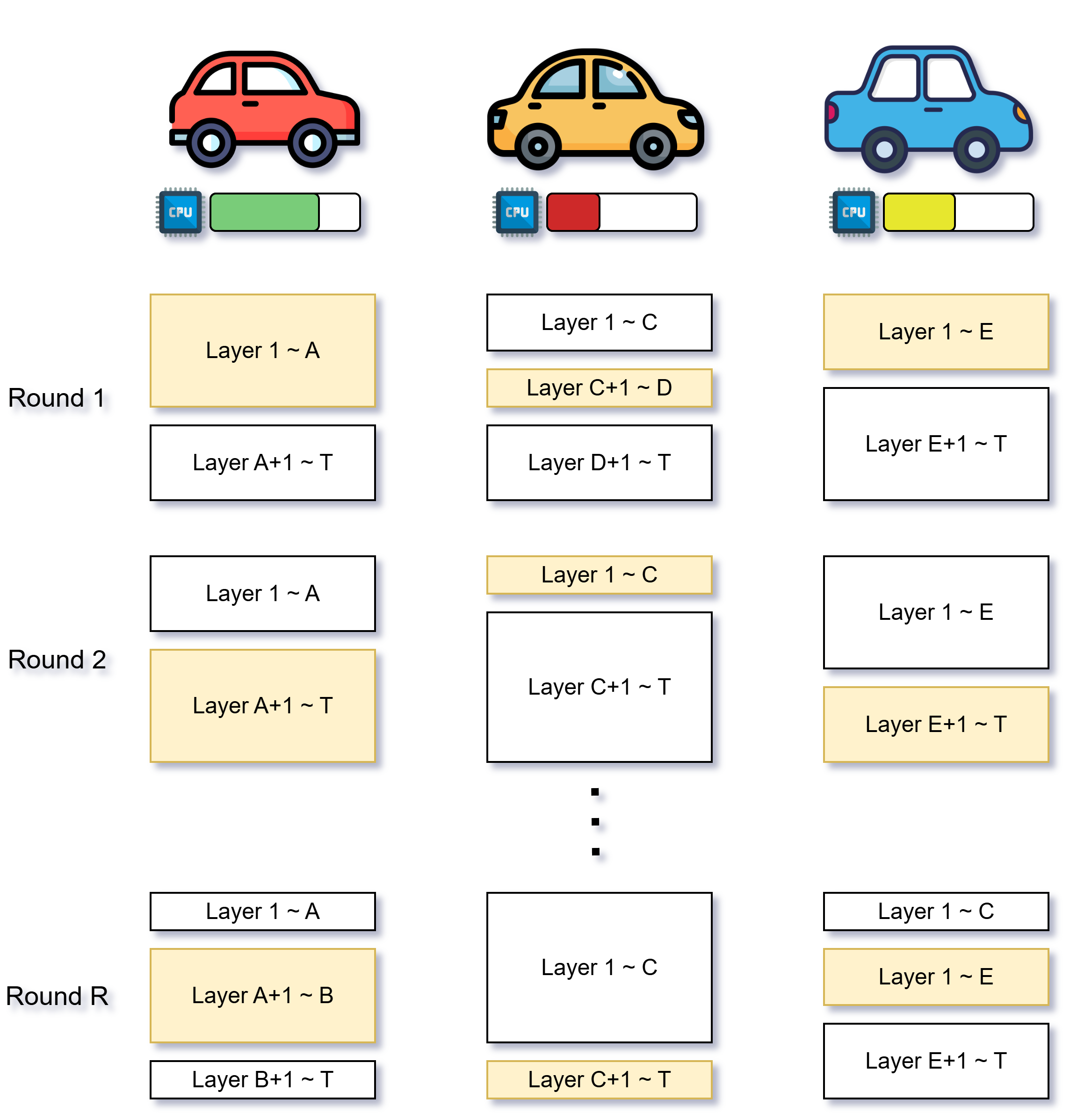
In this paper, we propose an FL scheme in which each vehicle selects the layer interval to be trained, in order to reduce the aggregation delay and to alleviate the data bias problem. The main contributions of this paper are summarized as follows.
• Through partial training of a contiguous layer interval that can be completed within a given time, vehicles with different computational capabilities complete training within the same time without waiting for slow vehicles.
• We propose an interval selection method in which each vehicle, based on its per-layer training records, selects with a higher probability the intervals containing layers that have been trained less frequently than others, so that the data of the vehicle are reflected evenly in the global model.
• We evaluate the proposed scheme on a real-world driving dataset and confirm that the aggregation delay is reduced compared with conventional FL and that the data bias problem is alleviated compared with existing partial training schemes.
The remainder of this paper is organized as follows. Section II reviews related work. Section III describes the system model and the proposed scheme. Section IV presents the simulation results, and Section V concludes the paper.
II. Related Work
To address the increase in aggregation delay caused by the long training time of vehicles with limited computational capability in FL, partial training, in which only a subset of the model layers is trained, has been studied [2]-[5]. This section reviews partial training schemes according to how the positions of the layers to be trained are determined.
A. Schemes with a Fixed Training Start Position
In these schemes, a device trains from the head up to the layer permitted by its computational capability. SALF [2] performs training from the head for a given time and then updates the model by aggregating each layer over the devices that trained it. FedOLF [3] determines the number of layers to be frozen in consideration of the device capability and trains only the remaining layers on the head side. In both schemes, devices with limited computational capability train only from the head up to a certain layer. Hence, the remaining layers of the body are trained only on the data of high-capability devices and become biased toward those data.
B. Schemes that Select the Training Position
In these schemes, the positions of the layers trained by a device change in every round. CoCoFL [4] determines, in every round, a set of candidate intervals that can be trained under the computation, communication, and memory constraints, and then randomly selects one interval from the candidates for training. FedRA [5] randomly selects, in every round, as many layers as the device can handle, and the selected layers need not be contiguous. In both schemes, devices with limited computational capability can also train layers of the body that are not adjacent to the head. However, since the layers previously trained by a device are not considered, it is difficult for its data to be reflected evenly in the model.
Similar to CoCoFL [4], this paper trains a contiguous layer interval that can be completed within a deadline; however, the interval is not selected uniformly at random but according to per-layer training records. The selection probability of an interval trained in the previous round is decreased and then gradually restored, so that the intervals are selected evenly.
III. Proposed Scheme
A. Problem Formulation
We consider an FL system consisting of K vehicles and a single server. The set of vehicles is denoted by K={1,…,k}. Vehicle k trains a classification model that recognizes the types of objects using its local dataset D_k, which consists of n_k images collected while driving. Since the environments in which vehicles mainly travel differ, the distribution of the local dataset varies across vehicles. An on-device AI device serves as the server; it does not participate in training and only aggregates the local model parameters transmitted by the vehicles. The objective of FL is formulated as [1]
where L_k^w denotes the loss of vehicle k on its local dataset. Training proceeds over T rounds. In round t, the server distributes the global model w^t to all vehicles, and each vehicle performs local training on its local dataset for E epochs and then transmits the trained local parameters to the server. The server aggregates the received local parameters to obtain w^(t+1). Since the server performs aggregation only after all vehicles have completed training and transmission, the aggregation delay of a round is determined by the slowest vehicle.
Figure 1. System model of the proposed scheme
B. Time Model of a Round
The model consists of a body, which extracts features, and a head, which is the classification layer. The model is divided into L layer units in order from the input and is denoted by w={w_1,…,w_(L}). Let q_l denote the number of parameters of unit l and C_l the forward computation cost of unit l for a single data sample. In each round, a vehicle trains a contiguous layer interval [i,j] (1≤i ≤j ≤L) and keeps the layers outside the interval fixed to the values received from the server. The interval trained by vehicle k in round t is denoted by [i_k^t,j_k^t], and training the entire model corresponds to [1,L].
Training the interval [i,j] requires a forward pass over the entire model, the backward propagation of the error from the head to the first unit of the interval, and the parameter update within the interval [4]. Hence, the training computation cost for a single data sample is given by
The computational speed of vehicle k in round t is expressed as a ratio relative to the fastest vehicle and is denoted by s_k^t∈(0,1]. Let D denote the time required for a vehicle with speed 1 to train the entire model [4]. Since the training time is proportional to the computation cost and inversely proportional to the computational speed, when all vehicles train the entire model, the training time of the slowest vehicle becomes D/min┬k〖s_k^t 〗, and the other vehicles must remain idle for the remaining time after completing their training. In contrast, if each vehicle trains an interval satisfying the following condition, all vehicles complete training within D:
(3)\frac{C(i_k^t, j_k^t)}{C(1, L)} \le s_k^t
In this paper, D is referred to as the deadline, and the deadline applies only to the training time.
A vehicle that has completed training transmits only the local parameters of the selected interval over the LTE uplink, and the vehicles in the same cell share the uplink capacity R. With each parameter represented by 32 bits, the completion time of round t is the sum of the training time τ_cmp^t and the upload time, which is given by
In this paper, τ^t is used as the measure of the aggregation delay. Since the global model is distributed in the same manner regardless of the interval to be trained, the time for updating and downloading the global model is not considered.
C. Motivation
In general, multiple intervals satisfy (3). For a vehicle with speed s, the maximal intervals among those satisfying (3) are referred to as candidate intervals [4], and their set is denoted by Α(s). A vehicle with speed 1 has a single candidate interval, [1,L]. Since the forward pass must be performed over the entire model regardless of the interval to be trained, the fraction of layers that a vehicle with limited computational speed can train is smaller than its speed ratio. Moreover, according to (2), the farther the first unit of an interval is from the head, the more computation is required for backward propagation; hence, candidate intervals farther from the head are shorter.
D. Proposed Scheme
In the proposed scheme, each vehicle maintains a training record for each layer unit and, based on these records, selects with a higher probability the candidate intervals that contain less frequently trained layers.
1) Interval Selection: Vehicle k maintains a record k_(k,l)^t for layer unit l, which is initialized as h_(k,l)^1=0. In round t, vehicle k obtains the candidate set Α(s_k^t) corresponding to its speed and computes the average record of the layers included in each candidate interval a=[i,j] as
A candidate interval with a smaller average record is selected with a higher probability, and in the first round, in which all records are zero, all candidate intervals have the same probability. The vehicle selects the interval [i_k^t,j_k^t] according to this probability and updates only the layers within the interval by stochastic gradient descent with learning rate η.
2) Record Update: After completing local training, a vehicle multiplies all records by a decay factor β∈(0,1) and then adds 1 to the records of the layers trained in the current round:
Accordingly, once a layer is trained, the selection probability of the intervals containing that layer decreases; if the layer is subsequently not trained for many rounds, its record decays and the selection probability is gradually restored. A larger decay factor β retains the past training history for a longer period.
3) Aggregation: A vehicle transmits the parameters of the trained interval together with the interval [i_k^t,j_k^t] to the server. The server obtains the set of vehicles that trained layer unit l, K_l^t={k∈K: i_k^t≤l ≤ j_k^t}, and for each layer unit, averages only the parameters of the vehicles that trained that unit in proportion to their data sizes [5]:
where w_(k,l)^t denotes the parameters of layer unit l of vehicle k after local training in round t. The overall framework is summarized in Algorithm 1. Since interval selection and record keeping are managed by the vehicles, the server does not maintain per-vehicle records. The only additional values stored by a vehicle are the L records, and since there is at most one candidate interval per starting unit, the computation required for selection is proportional to L.
IV. Simulation
A. Simulation Setup
The simulation settings are listed in Table I. The vehicles are divided into three tiers, namely high, mid, and low, according to their computational speed, and the speed of each vehicle is set every five rounds to one of the base speed, the base speed minus 0.1, and the base speed plus 0.1, without exceeding 1.0. To reflect the situation in which the driving environment differs across vehicles, a classification dataset is constructed by cropping object regions from the driving images of BDD100K [6]; images from different environments are assigned to each tier, and the proportions of the object classes are then determined by a Dirichlet distribution [7]. All vehicles have the same number of training samples.
Table 1. Simulation settings
Parameter
Value
Number of vehicles
50 (high: 15, mid: 20, low: 15)
Base speed
High: 1.0, mid: 0.7, low: 0.5
Model
ResNet-18 [8] with GroupNorm [9], approx. 11.17 M parameters, L=18
The proposed scheme is compared with FedAvg [1], in which all vehicles train the entire model; SALF [2], in which training proceeds from the head up to the layer that can be completed within the deadline; and CoCoFL [4], in which the candidate intervals are selected with equal probability. For SALF, local training is extended to multiple epochs as in the other schemes, and for CoCoFL, quantization is not used and only the time constraint is applied. All results are averaged over three seeds.
The degree to which the data of a vehicle are reflected evenly across the layers is evaluated by the fairness index [10]. Let x_(k,l) denote the number of times vehicle k trains layer unit l over all rounds. The fairness index of vehicle k is defined as follows, and the average over each tier is reported:
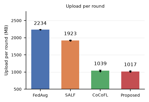
Fig. 2 shows the upload volume per round. In FedAvg, all vehicles transmit the entire model, resulting in 2,234 MB, whereas the proposed scheme requires 1,017 MB, which is 54.5% less than FedAvg. For SALF, the upload volume is 1,923 MB, a reduction of only 13.9%; this is because the parameters are concentrated in the layers close to the head, and thus a vehicle that trains from the head transmits a large amount of data even when the number of trained layers is small. The proposed scheme and CoCoFL use the same candidate intervals, and their upload volumes are therefore similar.
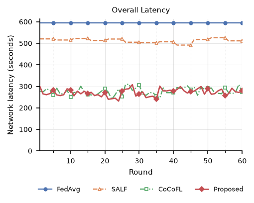
Figure 2. Upload Volume per roundFigure 3. Upload Latency per round
Fig. 3 shows the upload time in each round. FedAvg and SALF require approximately 596 s and 513 s, respectively, whereas the proposed scheme requires approximately 271 s, which is less than half that of FedAvg. The training time is equal to the deadline D for the proposed scheme, CoCoFL, and SALF, while it is longer for FedAvg because the slowest vehicle must be awaited. Consequently, the round completion time of the proposed scheme is also shorter than those of FedAvg and SALF.
C. Fairness of Layer Partial Training
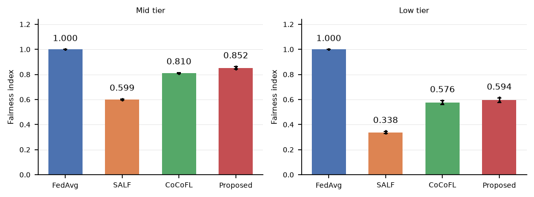
Fig. 4 shows the fairness index for each tier. The index of FedAvg is 1 because all layers are trained in every round; however, as shown above, its round time is the longest. Among the partial training schemes, the proposed scheme achieves the highest index. In the mid tier, the proposed scheme attains 0.852, which is higher than 0.599 for SALF and 0.810 for CoCoFL; in the low tier, it attains 0.594, which is also higher than 0.338 for SALF and 0.576 for CoCoFL. SALF yields the lowest index since only the layers close to the head are trained. In CoCoFL, the candidate intervals are selected evenly, but the layers in which the intervals overlap are trained more frequently; the proposed scheme reduces this disparity by incorporating the per-layer training records. The index of the low tier is lower than that of the mid tier because vehicles with low speed cannot train the layers of the body close to the input within the deadline.
Figure 4. Fairness index of layer partial training for each tier
D. Accuracy
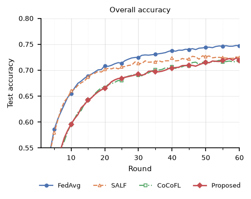
Fig. 5 shows the accuracy on the entire test set over the rounds. At round 60, FedAvg achieves an accuracy of approximately 75%, and the three schemes employing partial training achieve approximately 72%. The accuracy of the proposed scheme is comparable to that of CoCoFL and is approximately 3 percentage points lower than that of FedAvg, which trains the entire model. In the early stage of training, SALF, which trains the layers close to the head in every round, converges faster than the proposed scheme, but the gap narrows as the rounds proceed. Since the upload time per round of the proposed scheme is less than half that of FedAvg, more rounds can be performed within the same period of time.
Figure 5. Test accuracy comparison of the schemes
V. Conclusion
In this paper, we proposed an interval selection scheme for FL with vehicles of different computational resources, which reduces the aggregation delay while reflecting the data of slow vehicles evenly in the model. In the proposed scheme, each vehicle trains only a contiguous layer interval that can be completed within the deadline and, by maintaining per-layer training counts, selects with a higher probability the intervals containing less frequently trained layers. Since interval selection and record management are performed by the vehicles, the server only performs aggregation. In simulations on a real-world driving dataset, the proposed scheme reduced the upload time per round by approximately 55% compared with full-model training and achieved higher layer-wise training fairness than existing partial training schemes.
However, the accuracy of the proposed scheme was comparable to that of the scheme with random interval selection, and a limitation remains in that vehicles with low speed cannot train the layers of the body close to the input within the deadline. In future work, we plan to investigate methods that enable low-speed vehicles to contribute to the training of the layers close to the input, as well as interval selection methods that translate layer-wise training fairness into accuracy improvement. We also plan to extend the scheme by taking vehicle mobility into account.
VI. Acknowledgment
This work was supported by the 2026 National University Development Project funded by the Ministry of Education, Republic of Korea, and this work was supported by the Commercialization Promotion Agency for R&D Outcomes(COMPA) grant funded by the Korean Government(Ministry of Science and ICT). (RS-2023-00304695)
References
[1] MCMAHAN, Brendan, et al. Communication-efficient learning of deep networks from decentralized data. In: Artificial intelligence and statistics. Pmlr, 2017. p. 1273-1282.
[2] LANG, Natalie; COHEN, Alejandro; SHLEZINGER, Nir. Stragglers-aware low-latency synchronous federated learning via layer-wise model updates. IEEE Transactions on Communications, 2024, 73.5: 3333-3346.
[3] NIU, Ziru, et al. Energy and Memory-Efficient Federated Learning With Ordered Layer Freezing. IEEE Transactions on Mobile Computing, 2025.
[4] PFEIFFER, Kilian, et al. CocoFL: Communication-and computation-aware federated learning via partial NN freezing and quantization. arXiv preprint arXiv:2203.05468, 2022.
[5] SU, Shangchao; LI, Bin; XUE, Xiangyang. Fedra: A random allocation strategy for federated tuning to unleash the power of heterogeneous clients. In: European Conference on Computer Vision. Cham: Springer Nature Switzerland, 2024. p. 342-358.
[6] YU, Fisher, et al. Bdd100k: A diverse driving dataset for heterogeneous multitask learning. In: 2020 IEEE/CVF conference on computer vision and pattern recognition (CVPR). IEEE, 2020. p. 2633-2642.
[7] HSU, Tzu-Ming Harry; QI, Hang; BROWN, Matthew. Measuring the effects of non-identical data distribution for federated visual classification. arXiv preprint arXiv:1909.06335, 2019.
[8] HE, Kaiming, et al. Deep residual learning for image recognition. In: Proceedings of the IEEE conference on computer vision and pattern recognition. 2016. p. 770-778.
[9] WU, Yuxin; HE, Kaiming. Group normalization. In: Proceedings of the European conference on computer vision (ECCV). 2018. p. 3-19.
[10] JAIN, Rajendra K., et al. A quantitative measure of fairness and discrimination. Eastern Research Laboratory, Digital Equipment Corporation, Hudson, MA, 1984, 21.1: 2022-2023.